
Math at Uniswap V2
Published:
Uniswap V2 is one of the most studied smart contracts ever deployed. At its core sits a single line of mathematics:
\[x \cdot y = k\]
No order book. No matching engine. Just two token reserves and a constant. This post unpacks exactly how that formula translates into the tokens you receive when you make a swap.

The math above started exactly where most understanding does — a notebook. Working through the algebra by hand is how the intuition forms: why the curve is a hyperbola, why large trades move the price more, why the fee fits so cleanly into the same formula.
This post is the bridge from those handwritten steps to real practice. To make it fully concrete, I am currently building an interactive AMM calculator — plug in your own reserves and trade size, and watch $\Delta y$, slippage, and price impact update live. It will sit alongside this post as the hands-on counterpart to the derivation.
What is an AMM?
A traditional exchange matches buyers with sellers through an order book. An Automated Market Maker (AMM) replaces that entirely — a smart contract holds reserves of two tokens and prices every trade algorithmically.
Uniswap V2’s pool has four actors:
| Actor | Role |
|---|---|
| Liquidity pool | Smart contract holding reserves of token X and token Y |
| Liquidity providers (LPs) | Deposit tokens, receive LP tokens representing their share |
| Traders | Swap one token for another by paying a fee |
| Fee | $f = 0.003$ (0.3 %), distributed to LPs on every swap |
The constant product formula
The heart of Uniswap V2 is the constant product formula:
$$x \cdot y = k$$
where:
- \(x\) = reserve of token X in the pool
- \(y\) = reserve of token Y in the pool
- \(k\) = constant (remains the same before and after the swap, ignoring fees)
$k$ must hold before and after every swap (ignoring fees for now).
The curve $x \cdot y = k$ is a hyperbola. The spot price of X in terms of Y is the negative slope of the curve at any given point — so price changes continuously as reserves move.

When a trader deposits $\Delta x$ tokens X into the pool:
- The reserve of X rises from $x_0$ to $x_0 + \Delta x$
- To keep $k$ constant, the reserve of Y must fall from $y_0$ to $y_0 - \Delta y$
- The trader receives $\Delta y$ tokens Y
Deriving the output formula $\Delta y$
Starting point
Initial pool state satisfies the invariant:
\[x_0 \cdot y_0 = k\]After the swap, the new state must satisfy the same constant:
\[(x_0 + \Delta x)(y_0 - \Delta y) = k\]Step 1 — Equate
Since both expressions equal $k$:
\[x_0 \cdot y_0 = (x_0 + \Delta x)(y_0 - \Delta y)\]Step 2 — Divide both sides by $(x_0 + \Delta x)$
\[\frac{x_0 \cdot y_0}{x_0 + \Delta x} = y_0 - \Delta y\]Step 3 — Isolate $\Delta y$
\[\Delta y = y_0 - \frac{x_0 \cdot y_0}{x_0 + \Delta x}\]Step 4 — Common denominator
\[\Delta y = \frac{y_0(x_0 + \Delta x) - x_0 \cdot y_0}{x_0 + \Delta x}\] \[\Delta y = \frac{\cancel{x_0 y_0} + \Delta x \cdot y_0 - \cancel{x_0 y_0}}{x_0 + \Delta x}\]Step 5 — Cancel and simplify
The $x_0 y_0$ terms cancel:
$$\Delta y = \frac{\Delta x \cdot y_0}{x_0 + \Delta x}$$
This is the amount of token Y received when depositing $\Delta x$ of token X, without the fee.
Numerical check
Take $x_0 = 2$, $y_0 = 6$, $k = 12$, $\Delta x = 4$:
\[\Delta y = \frac{4 \times 6}{2 + 4} = \frac{24}{6} = 4\]The pool moves from $(2,\, 6)$ to $(6,\, 2)$, and $6 \times 2 = 12 = k$ ✓
Including the fee: factor $(1 - f)$
In practice Uniswap deducts the fee before processing the swap. If the trader sends $\Delta x$, only $(1 - f) \cdot \Delta x$ effectively enters the pool calculation; the remaining $f \cdot \Delta x$ accrues to the LPs.
Substituting $(1 - f)\Delta x$ for $\Delta x$ in the formula above:
\[(x_0 + (1-f)\Delta x)(y_0 - \Delta y) = x_0 \cdot y_0\]Following identical algebra:
\[\boxed{\Delta y = \frac{(1 - f)\cdot \Delta x \cdot y_0}{x_0 + (1 - f)\cdot \Delta x}}\]where $f = 0.003$ for Uniswap V2.
Numerical example
Pool: $x_0 = 100\text{ ETH}$, $y_0 = 200{,}000\text{ USDC}$. Trader swaps $\Delta x = 1\text{ ETH}$.
\[\Delta y = \frac{0.997 \times 1 \times 200{,}000}{100 + 0.997 \times 1} = \frac{199{,}400}{100.997} \approx 1{,}974.3\text{ USDC}\]The initial spot price was $200{,}000 / 100 = 2{,}000$ USDC/ETH. The trader receives only $\approx 1{,}974.3$ USDC/ETH — the gap comes from slippage (price impact) plus the 0.3 % fee.
Marginal price and slippage
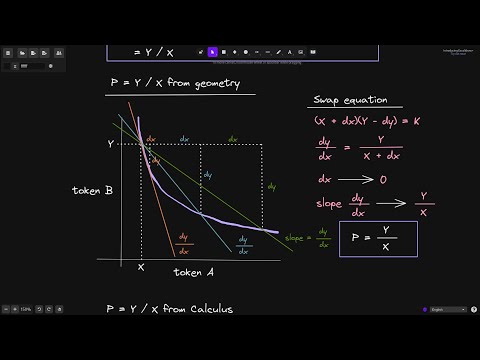
The instantaneous price of X in terms of Y at any point on the curve is:
\[P = -\frac{dy}{dx} = \frac{y}{x}\]This is the derivative of $y = k/x$. The price is never fixed — it shifts with every unit traded. The bigger the trade relative to the pool, the more the price moves against the trader.

The dashed line is the ideal price (no slippage). The real AMM curves fall below it — and the gap widens as $\Delta x$ grows. This is price impact: large trades are penalised by the curve’s curvature.
Key formula summary
| Concept | Formula | Note |
|---|---|---|
| AMM invariant | $x \cdot y = k$ | Holds before and after every swap |
| Output (no fee) | $\Delta y = \dfrac{\Delta x \cdot y_0}{x_0 + \Delta x}$ | Exact tokens received |
| Output (with fee) | $\Delta y = \dfrac{(1-f)\Delta x \cdot y_0}{x_0 + (1-f)\Delta x}$ | $f = 0.003$ in Uniswap V2 |
| Marginal price | $P = \dfrac{y}{x}$ | Instantaneous, no slippage |
Conclusion
Uniswap V2 shows that a single algebraic constraint — $x \cdot y = k$ — is enough to build a fully autonomous exchange. The $\Delta y$ formula we derived lets any trader calculate their exact output before executing a swap. The $(1 - f)$ factor folds the protocol fee into the same equation, rewarding liquidity providers and making the system self-sustaining.
The elegance is in the simplicity: no order matching, no counterparty risk, no off-chain infrastructure — just a constant and the blockchain.
All the math covered here — the constant product invariant, the $\Delta y$ derivation, the fee factor — also underpins something worth highlighting: how to calculate the spot price of a constant product AMM. The same formula, a different lens.
Smart Contract Programmer has an excellent series on this. Every video is clear, precise, and directly useful if you are working through the DeFi primitives from the ground up. The episode below goes straight into the spot price calculation and is a great complement to this post:
Smart Contract Programmer · Constant Product AMM Spot Price